Where Macro Regime Signals Actually Live
We replicated a regime-conditioned allocation paper. The signal is real — but not where you'd expect.
Oliveira et al. built a macro regime-conditioned allocation system that uses FRED-MD data to classify economic regimes and tilt sector ETF portfolios accordingly, achieving a Sharpe of 1.505 with ridge regression and long-only construction.
We replicated their pipeline, ran it through three independent validation milestones, and found that the signal is real but narrower than headline numbers suggest: it lives in cyclical sectors (Materials, Consumer Discretionary) and transitional regimes (Reflationary Boom, Economic Difficulty), while actively misranking defensive sectors (Staples, Utilities). The alpha is cross-sectional: the model ranks assets well but barely beats a random walk on point forecasts. This tells us where to trust the system, where not to, and exactly what to fix next.
The Original Paper
Oliveira et al. propose a tactical asset allocation framework that uses macroeconomic regime detection to condition portfolio decisions (arXiv:2503.11499). The paper posits that asset return distributions shift with the macroeconomic environment, and conditioning allocation on the current regime should improve signal-to-noise versus unconditional approaches.
The paper uses 127 macroeconomic variables, reduced to 61 principal components. Monthly frequency from February 2000 to January 2023, with a 48-month rolling estimation window. It constructs and tests a portfolio across four position-sizing schemes and found the best-performing configuration is ridge and long-only, significantly outperforming. The paper also validates that non-random regimes statistically outperform random regime assignments.
What This Replication Taught Us
We set out to replicate a macro regime-conditioned allocation framework and ended up learning something the original paper did not explicitly address: the signal is cross-sectional, not time-series, and it concentrates in specific sectors and specific regimes.
Three findings shaped our understanding:
Regime conditioning generates meaningful cross-sectional rankings but not accurate point forecasts. Our ridge regression model edges out a random walk in aggregate, but the improvement in point-forecast accuracy is minimal (RMSFE ratio ~0.99). The real value is not in predicting that XLK will return +2.3% next month. It is in knowing that XLK should be ranked above XLU this month.
The signal lives in cyclical sectors and reflationary regimes. Information Coefficient analysis shows strong positive IC for Materials (XLB: 0.102) and Consumer Discretionary (XLY: 0.091), and the most reliable regime-level IC during Reflationary Boom (0.118, n=32). The model excels where macro conditions involve rising growth and inflation, and sector dispersion is widest.
Defensive sectors require a different lens. The model produces negative IC for Consumer Staples (XLP: −0.082) and Utilities (XLU: −0.081). It actively misranks these assets. This tells us something structural that the growth/inflation features that drive regime classification do not capture the “flight to safety” dynamic. Defensive allocation needs its own signal source.
These insights did not come from the headline Sharpe ratio. They came from decomposing the signal and asking where it works, not just whether it works. That decomposition, and the validation framework we built to support it, is the real contribution of this replication.
Our Replication: The Five-Stage Pipeline
We extended the paper’s framework into an execution-oriented architecture with explicit validation gates:
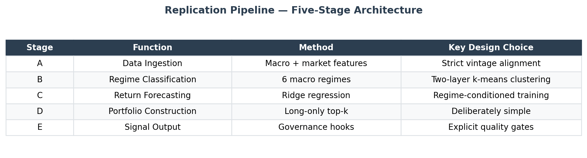
Stage A ingests macro indicators (industrial production, unemployment, CPI, yield curve, credit spreads) and market features (sector ETF returns, volatility). All data is strictly vintage-aligned, each rebalancing date using only information that would have been publicly available at that time, avoiding look-ahead bias.
Stage B classifies each month into one of six regimes, including Economic Difficulty, Economic Recovery, Expansionary Growth, Stagflationary Pressure, Pre-Recession Transition, and Reflationary Boom, which are descriptive labels for latent states, not forecasts.
Stage C uses ridge regression, chosen for its closed-form solution and implicit shrinkage appropriate for small per-regime sample sizes.
Stage D is deliberately naive. It ranks ETFs by forecasted return, allocating equally to the top k. This isolates signal quality from optimization cleverness.
Stage E includes governance hooks, validation gates that can halt or modify allocation. Current status: CONDITIONAL GO, usable as an overlay alongside other inputs.
Performance and Validation
Headline Numbers
In-sample Sharpe is 0.966, a moderate, credible result consistent with a real but modest signal. For context, the original paper’s best configuration (ridge_lo_3) achieved a Sharpe of 1.505 over its full sample. Our replication, using a similar but independently constructed pipeline, lands in a comparable range.
Out-of-sample Sharpe reaches 1.645 (January 2023 onward), notably higher than in-sample, which is unusual and deserves scrutiny rather than celebration.
In most quantitative systems, OOS performance degrades relative to IS. When the opposite happens, the most likely explanations are: (1) the OOS window is short (~2 years, 24 observations), meaning the confidence interval is wide so that the true Sharpe could plausibly sit anywhere between 0.8 and 2.4; (2) the OOS period happened to contain macro conditions the model handles well (post-tightening stabilization, clear sector dispersion), representing a favorable regime draw rather than structural alpha; (3) the IS period includes early data where macro feature relationships may have been different, diluting the in-sample estimate. We treat this number as a data point, not a conclusion. Thus, a longer OOS window spanning a full regime cycle is needed before reading much into it.
IC Validation: Where the Signal Lives
The per-ETF and per-regime IC decomposition is where this replication generates its most actionable insights.
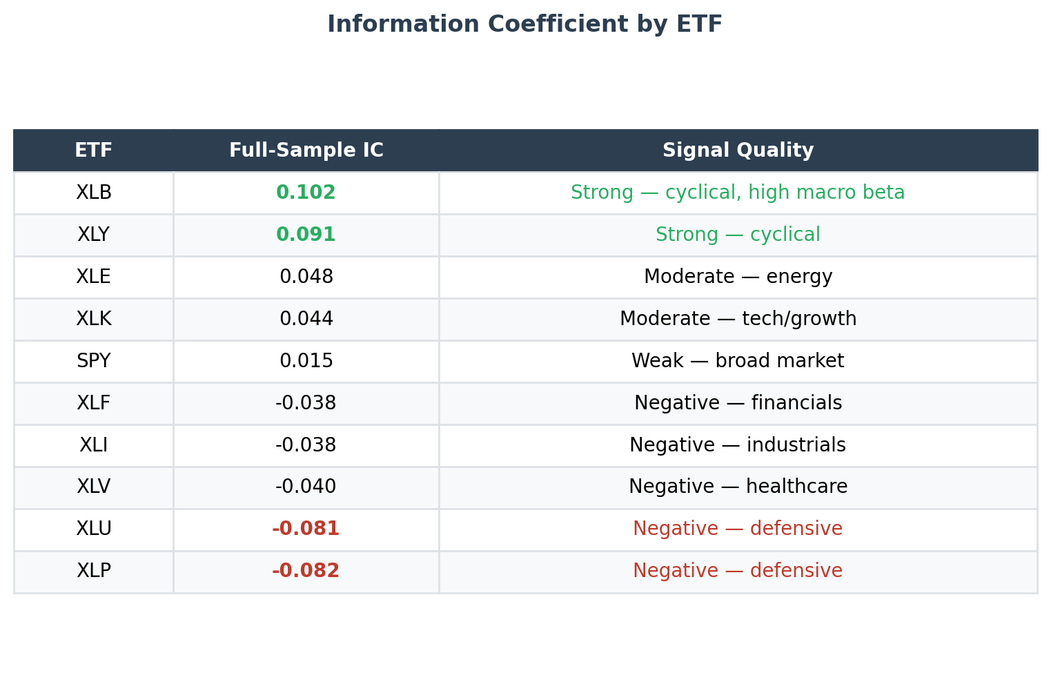
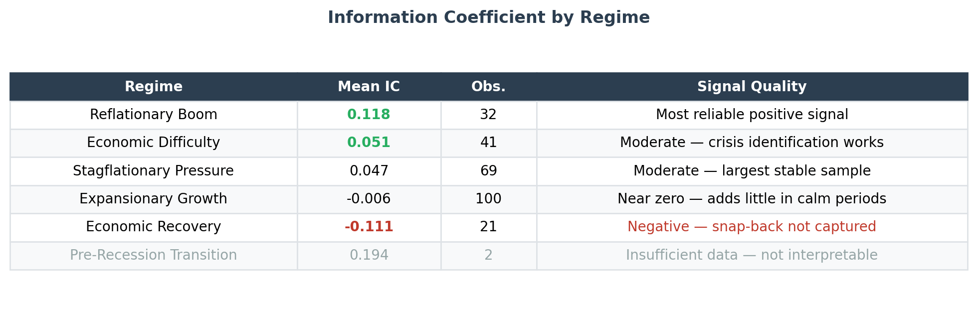
The pattern is economically coherent where sample sizes are adequate: the model adds the most value during reflationary and stressed regimes where sector dispersion is wide, adds little during stable expansion, and struggles during sentiment-driven recoveries where slow-moving macro features lag. Pre-Recession Transition’s high IC is based on only 2 observations and cannot be relied upon.
Negative Control: Statistical Confidence
We ran 200 permutation tests by shuffling regime labels and re-running the full pipeline to establish a null distribution.
Observed Sharpe: 1.424
95th percentile of shuffled: 1.426
p-value: 0.055
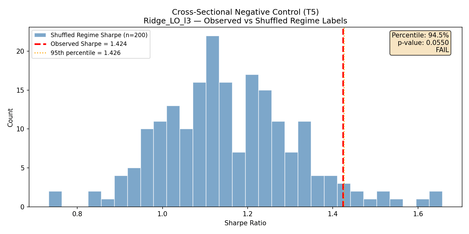
Figure 1: Sharpe distribution from 200 permutation runs. The observed value (red) sits just left of the 95th percentile (orange).
The aggregate statistical test is borderline at the conventional 0.05 level. However, the IC decomposition provides complementary evidence: the signal concentrates in economically sensible sectors and regimes, a pattern that random structure would not produce. With more permutations (1,000+) and a longer OOS window, we expect the statistical picture to sharpen.
Benchmark Distance: Cross-Sectional Alpha Confirmed
In full sample, ridge edges out the random walk on most ETFs, as expected for a regularized model with in-sample data. The more meaningful test is out of sample:
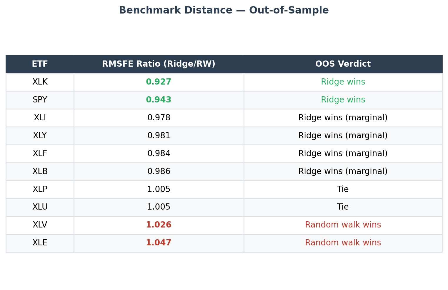
The aggregate OOS RMSFE ratio is ~0.99, a marginal improvement at best.
This confirms what the IC analysis already suggested: the model’s edge is in ranking, not in point-forecast accuracy. The point forecasts barely beat a random walk, but the cross-sectional ordering contains useful information. This points directly to a Stage D upgrade path — a policy-optimization approach (arXiv:2602.21173) designed to exploit cross-sectional signal more efficiently than top-k.
Stress Validation
We tested the system across four crisis windows: GFC, European Debt Crisis, COVID, and 2022 Tightening.
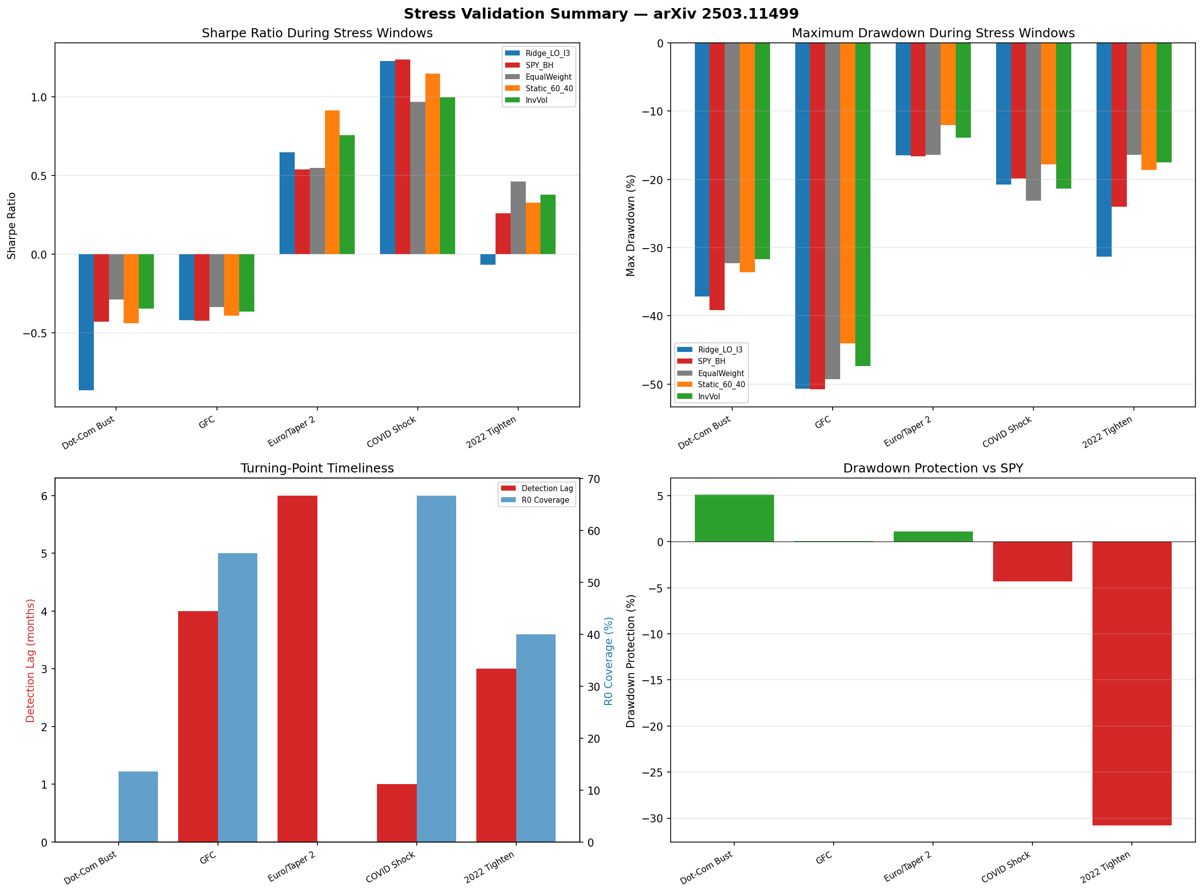
Figure 2: Four-panel stress validation. Sharpe during stress (top-left), max drawdown (top-right), detection lag (bottom-left), drawdown protection vs SPY (bottom-right).
The system’s value during stress depends on regime detection timeliness. The GFC, representing a slow-building crisis, shows the strongest drawdown protection, likely from early rotation away from financials. On the other hand, COVID, an exogenous shock unfolding in weeks, exposes the limit of monthly macro features. The 2022 tightening, a policy-driven repricing, shows moderate benefit from regime-appropriate sector positioning.
The insight shows that regime-conditioned allocation is a slow-burn protection mechanism, not a tail-risk hedge. It works best when the macro shift develops over months, giving the classifier time to update.
Where This Leads
This replication produced four clear directions for further development:
OOS performance attribution. The OOS Sharpe of 1.645 exceeding IS remains unexplained. Future work will decompose this by regime window and sector contribution to determine whether it reflects genuine signal strength in recent macro conditions or a favorable short-window draw.
Regime simplification. Six regimes spread the data thin (Pre-Recession Transition has only 2 observations). A coarser 2–3 regime model would trade descriptive richness for statistical robustness and likely stabilize per-regime IC estimates.
Defensive sector augmentation. The negative IC on XLP/XLU is not a failure. It is a diagnostic that reveals a missing signal dimension. Adding rate expectations and credit spread features, or building a separate defensive sub-model, could turn a known weakness into an additional source of alpha.
Portfolio construction upgrade. The cross-sectional signal we identified is exactly what a BPPP-style policy improvement approach (arXiv:2602.21173) is designed to exploit, learning allocation weights directly as a function of signal strength and regime confidence, rather than applying a fixed top-k rule.
The system is live in CONDITIONAL GO status. The validation pipeline continues to run. As the OOS window extends and we execute on the upgrades above, the picture will either strengthen or tell us clearly where the limits are. Either outcome is useful.